Discretizing Baby Sleep Timeseries with Pandas

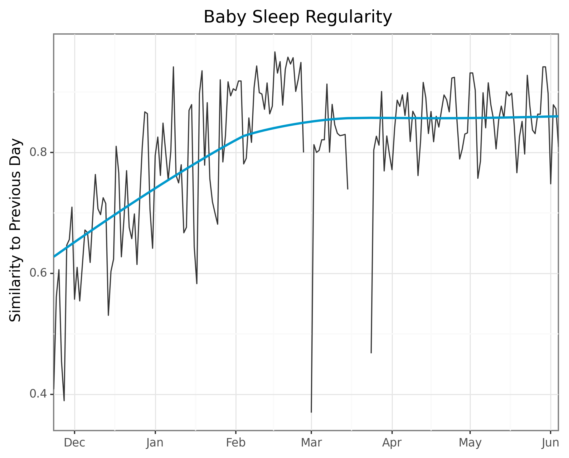
This is part of a series on visualizing baby sleep data with Python and R. All code is in this repository.

• Visualizing Baby Sleep Times in Python
• Recreating the ‘Most Beautiful Data Visualization of All Time’
• Night and Day, Python and R: Baby Sleep Data Analysis with Siuba
• Discretizing Baby Sleep Timeseries with Pandas

This post shows a few methods for turning a representation of time as a series of periods into a binary vector for use in clustering or other data anslysis.

Motivation: A newborn’s sleep is chaotic before transitioning to a more regular schedule. You can clearly see this in my child’s sleep behavior in the graph below.

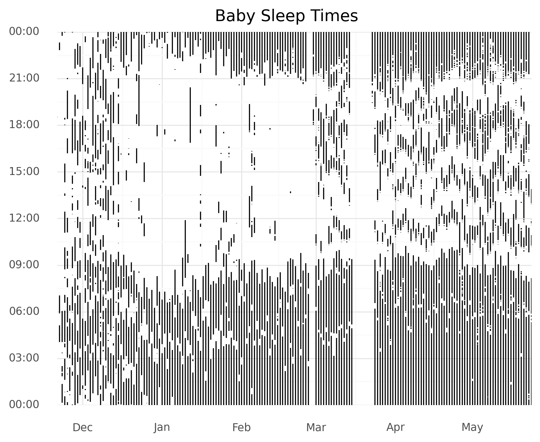
I decided I’d try to quantify this shift from more random to more regular over time. Additionally, I wanted to do some clustering to look at when certain transitions occurred and to make some pretty graphs!

My first benchmark here is to compare days to see how similar they are. I decided to represent each day as a vector and then run cosine similarity. Start simple! To do this, however, I need to represent days as vectors. I decided to settle on breaking days into 15 minute increments. The first item in the vector would be a 1 if the baby was asleep in the first 15 minutes of the day and a 0 otherwise. This would repeat for the rest of the day, so we’ll have a vector of length 24 hours * 4 time-periods / hour = 96. For time time periods with some sleep and some awake, we’ll just call it entirely asleep.

Let’s dive into some Pandas code.

Preliminaries

As I showed in my first post, our data looks like this:

In [207]: !head all_snoo_sessions.csv
start_time,end_time,duration,asleep,soothing
2019-11-21T18:30:38,2019-11-21T18:31:58,80,80,0
2019-11-22T04:03:32,2019-11-22T05:07:27,3835,2422,1413
2019-11-22T05:53:04,2019-11-22T05:54:07,63,36,27

Basically, each row is a period of time where the baby was asleep.

First, we import necessary libraries, add some constants, and do some type conversions and add extra columns for convenience.

import datetime as dt

import numpy as np
from palettable.lightbartlein.diverging import BlueGray_2
import pandas as pd
from plotnine import *
from scipy.spatial import distance


# Constants
COLOR_VALUES = BlueGray_2

ONE_SECOND = dt.timedelta(seconds = 1)
FIFTEEN_MINUTES = dt.timedelta(minutes = 15)
ONE_DAY = dt.timedelta(days = 1)


# Read in data
df = pd.read_csv("sleep_data.csv")


# Break out dates and times.
df["start_datetime"] = pd.to_datetime(df["start_time"])
df["end_datetime"] = pd.to_datetime(df["end_time"])
df["start_time"] = df["start_datetime"].dt.time
df["end_time"] = df["end_datetime"].dt.time
df["start_date"] = df["start_datetime"].dt.date

Discretize Time Periods

Pandas has a powerful resample function which is great for our use case. However, to use it, we need our data to be formatted as a Series with a time index.

You could think of this next block of code as turning our “wide” dataframe with multiple observations per row (when did baby wake up? When did baby sleep?) into a “long” dataframe, with one observation per row (when did baby do something, and what was it?). As always, Hadley Wickham’s paper is great for thinking about data formats.

## Part 1: Combine start and end times into one series.
start_times = df[["start_datetime"]].copy()
start_times.columns = ["timestamp"]  # Rename column.
start_times["is_asleep"] = 1

end_times = df[["end_datetime"]].copy()
end_times.columns = ["timestamp"]  # Rename column.
end_times["is_asleep"] = 0

all_times = pd.concat([start_times, end_times]).sort_values("timestamp")

# Handle an annoying issue where duplicate timestamps breaks resampling later.
all_times["timestamp"] = np.where(all_times.timestamp == all_times.timestamp.shift(-1),
                                  all_times.timestamp + ONE_SECOND,
                                  all_times.timestamp)

all_times = all_times.set_index("timestamp")

Next up, I’ll use the resample method in two different ways. One is easy to write and think about, but much slower.

Method 1: Upsample then Downsample

disc_1 = all_times.resample("1S").ffill().resample("15min").max()

In this version, we resample to a one second granularity and forward fill. We follow this up by resampling to a 15 minute granularity and taking the max value within that 15 minute time window.

In a bit more detail, all_times.resample("1S") gives us a Series with a row for every second between our start and end times. The value at the series will be 1 or 0 at the timestamps present in all_times, and null everywhere else. The .ffill() call then fills every null with the first non-null value before it. The resample call will give us a new series with a row for each 15 minute time block. Finally, calling .max() on the resampled series means

A helpful way to think about resample([time granularity]).function() is sort of like a groupby: we group rows together based on the time windows, and then use the function to decide how to go from those rows to either a few rows (like in an aggregation) or many rows (via interpolation or some other method).

Because we’re making potentially a lot of rows, this uses lots of time and computation. But it’s super quick to write, and oftentimes for data scientists we only have to run code like this once or twice.

Method 2: Resample Twice and Combine

# Discretize Method 2: Combine max to get the right value, last + ffill to get fills
r = all_times.resample("15min")
r_last = r.last().fillna(method = "ffill")
r_max = r.max()
r_max[~r_max.isna().values] = 1  # If it contains a value, set it to 1, else leave null

disc_2 = r_max.combine_first(r_last).astype(int)

We’re doing two things here. First, let’s focus on r_last. We could think of the values in all_times as when we’re throwing an on/off, awake/asleep switch. Thus, for any time after we’ve set the switch to one, we want the value to be one. If baby fell asleep at 4:58pm and wakes up at 5:28pm, we want the 5:00pm and 5:15pm periods to be asleep as well. r.last() says when we have multiple rows in a time window, take the value of the last one. The .fillna(method = "ffill") then “pushes” that last value forward, replacing all nulls until it hits a That’s going to be correct for all the nulls it replaces, but sometimes incorrect for the window in which the value occurs. If baby fell asleep at 12:16am and woke up at 12:18am, we want the value to be asleep for the 12:15-12:30am window, and this will take the last value, awake.

So that’s why we need to use r_max. While r_last will be correct for all values that were null in the resampled array, r_max will be correct for all values taht were not null in the resampled array. If any value appears in the time window, then the baby was asleep at some portion of it. Thus, we set all these values to 1.

Finally, we cimply combine these two arrays with the combine_first method, which works similarly to a SQL coalesce and set the type to int.

Method Comparison

The first method is quick to write but slow to execute. The second method is more cumbersome but faster. How much faster? On my old laptop where I’m running this, method 1 took 3 seconds and method 2 took 68ms, so basically two orders of magnitude difference.

They do give the same result, as we can verify with:

assert disc_1.equals(disc_2)

Create Feature Vectors

The above code gave us one long time series broken into evenly spaced, 15 minute increments. Since we want to compare days, let’s now break apart that series into separate days. Again, I’l show two methods.

# Filter to full days
disc_1 = disc_1[(disc_1.index >= pd.to_datetime("2019-11-22"))
                & (disc_1.index < pd.to_datetime("2020-06-05"))]


num_periods = int(ONE_DAY / FIFTEEN_MINUTES)


# Featurize Method 1: Simply use a reshape
ftrs_1 = disc_1.values.reshape(len(disc_1) // num_periods, num_periods)

One option is to operate in “numpy” land by operating directly on the values. We figure out how big our vector should be, and reshape.

# Featurize Method 2: Use a pivot table
ftrs_2 = disc_1.reset_index()
ftrs_2["date"] = ftrs_2.timestamp.dt.date
ftrs_2["time"] = ftrs_2.timestamp.dt.time
ftrs_2 = ftrs_2.pivot(index="date", columns="time", values="is_asleep")

Another option is to turn our timeseries into a DataFrame, add some columns to break apart each day, and use the pivot method to rearrange everything. The pro of this method is we get to keep our data as a DataFrame with comprehensible column names. The downside is we’re now in Weird Pandas Multi-Index Multi-Column world, which I really dislike.

Again, we can verify the two are the same:

assert (ftrs_1 == ftrs_2).all(axis=None)

Distance Metric and Plotting

## Part 4: Compute cosine similarity between vectors
# Compute it. Cos Similarity = 1 - Cos Distance
similarity = [1 - distance.cosine(i, j) for i, j 
              in zip(ftrs_2.iloc[0:-1].values, ftrs_2.iloc[1:].values)]

Finally, we actually compute the cosine similarity, the easiest part of all of this. I did this by zipping the two lists of vectors with a one day offset.

Next I’ll plot using my favorite plotting library of the moment, plotnine. I use some custom colors because I thought they looked nice in my last post.

# Plot it!
plot = (ggplot(aes(x = "date", y = "similarity", group = 1), data=plot_df) 
  + geom_line(color = COLOR_VALUES.hex_colors[1])
  + scale_x_date(name="", date_labels="%b", expand=(0, 0)) 
  + ylab("Similarity to Previous Day")
  + geom_smooth(color = COLOR_VALUES.hex_colors[0])
  + theme_bw()
  + ggtitle("Baby Sleep Regularity")
  )
print(plot)
ggsave(
  plot,
  "fig/lineplot_time_cossimilarity.png",
  width=6.96, height=5.51, units="in", dpi=300
)

The trend does indeed appear to go from really dissimilar sleep to much more regular patterns!